
In my last post, we looked at using the sentiment of financial news as an indicator for stock trading. The method used was VADER, an out of the box sentiment analysis method that does not rely on machine learning and is simply a pre-weighted lexicon.
As previously discussed, we can improve upon the techniques used in that post.
The Data
The quality of our model is going to be constrained by the quality of our dataset. For this investigation, I’m using financial news data sourced from Kaggle that has been pre-labelled.
Constructing the Naive Bayes Classifier
A simple improvement over VADER should be that of the Naive Bayes Classifier.
Here’s the workflow we’ll follow:
- Load dataset
- Vectorize data
- Split data (80/20, train test, random_state=0 so as to allow reproducability)
- Initialize the NB classifer and fit
- Predict and measure accuracy
from sklearn.feature_extraction.text import CountVectorizer

news_pd = pd.read_csv("/kaggle/working/news_with_sentiment.csv")
news_pd = news_pd[:20000]

cv = CountVectorizer() # Convert text data to a vector as that is required for Naive Bayes
X = cv.fit_transform(news_pd['text']).toarray()
y = news_pd['sentiment'] # y = the variable we are trying to predict, in this case sentiment
# Split train and test data (80/20)
from sklearn.model_selection import train_test_split
X_train, X_test, y_train, y_test = train_test_split(X, y, test_size = 0.20, random_state = 0)

# Initialize the Gaussian Naive Bayes Classifier, then fit the data
from sklearn.naive_bayes import GaussianNB
classifier = GaussianNB()
classifier.fit(X_train, y_train)
GaussianNB(priors=None, var_smoothing=1e-09)
# Predict sentiment of our test data
y_pred = classifier.predict(X_test)

from sklearn.metrics import accuracy_score
score = accuracy_score(y_test, y_pred)
And now we can view the accuracy:
print(score)
0.56925
Roughly 57% accuracy. Not exactly stellar, we could potentially boost this by hyperparameter tuning but I think it’s best if we try another approach.
To improve on our Naive Bayes we can now try a Random Forest:
A random forest approach may reduce our errors, and improve our accuracy. Let’s give it a try using 20,000 rows of our data.
This is the workflow we’ll use for a random forest approach:
- Load dataset
- Remove stopwords, min_df=7 means the data is irrelevant if used in less than 7 documents, max_df of 0.8 means it also is irrelevant if used in more than 80% of documents
- Vectorize data (max_features is the max number of (frequent) words in vector form that will influence the sentiment)
- Split data (80/20, train test, random_state=0 so as to allow reproducability)
- Initialize the Random Forest classifer and fit
- Predict and measure accuracy
# Read in 20,000 headlines
news_pd = pd.read_csv("/kaggle/working/news_with_sentiment.csv")
news_pd = news_pd[:20000]

y = news_pd['sentiment']
from nltk.corpus import stopwords
from sklearn.feature_extraction.text import TfidfVectorizer

# Remove stopwords and vectorize the dataset
vectorizer = TfidfVectorizer(max_features=2500, min_df=7, max_df=0.8, stop_words=stopwords.words('english'))
processed_features = vectorizer.fit_transform(news_pd['text']).toarray()
# 80/20 data split
from sklearn.model_selection import train_test_split
X_train, X_test, y_train, y_test = train_test_split(processed_features, y, test_size=0.2, random_state=0)

# Fit our model with split data, starting with 450 estimators (450 decision trees)
from sklearn.ensemble import RandomForestClassifier

text_classifier = RandomForestClassifier(n_estimators=450, random_state=0)
text_classifier.fit(X_train, y_train)
RandomForestClassifier(bootstrap=True, ccp_alpha=0.0, class_weight=None,
                       criterion='gini', max_depth=None, max_features='auto',
                       max_leaf_nodes=None, max_samples=None,
                       min_impurity_decrease=0.0, min_impurity_split=None,
                       min_samples_leaf=1, min_samples_split=2,
                       min_weight_fraction_leaf=0.0, n_estimators=450,
                       n_jobs=None, oob_score=False, random_state=0, verbose=0,
                       warm_start=False)
# Predicting the sentiment of our test data
predictions = text_classifier.predict(X_test)


# Checking our accuracy
from sklearn.metrics import accuracy_score
print(accuracy_score(y_test, predictions))
0.93575
93.57% accuracy - A great improvement!
Hyperparameter Tuning (n_estimators):
It’s important to tune your model to get the best possible accuracy. Next, I’m going to run a trial of a large set of different input parameters for our random forest classifier’s number of estimators, and determine if we can gather any measurable gain in accuracy as a result.
Note: This can be achieved using in-built functions within sklearn such as GridSearchCV and RandomizedSearchCV, but I have chosen to do it manually and plot the results.
Here’s our workflow:
- Create an array of n_estimators we wish to trial
- Run through each permutation, store the resulting accuracy
- Plot the results
from sklearn.ensemble import RandomForestRegressor

estimators = [50, 100, 150, 200, 250, 300, 350, 400, 450, 500, 550, 600, 650, 700, 900, 1000, 1250, 1500, 2000]
accuracy = []

for estimator_num in estimators:
    # Fit and predict
    text_classifier = RandomForestClassifier(n_estimators=estimator_num, random_state=0)
    text_classifier.fit(X_train, y_train)
    predictions = text_classifier.predict(X_test)

    # Store accuracy
    from sklearn.metrics import accuracy_score
    accuracy.append(accuracy_score(y_test, predictions))


#Graph reported accuracy of various sets of estimators
import matplotlib.pyplot as plt

plt.plot(estimators, accuracy)
plt.ylabel('Accuracy')
plt.xlabel('Estimators')
plt.show()

print(estimators)
print(accuracy)
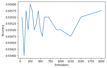
[50, 100, 150, 200, 250, 300, 350, 400, 450, 500, 550, 600, 650, 700, 900, 1000, 1250, 1500, 2000]
[0.9355, 0.934, 0.93575, 0.935, 0.936, 0.93575, 0.935, 0.93525, 0.93575, 0.935, 0.93475, 0.9355, 0.9355, 0.9355, 0.935, 0.935, 0.93475, 0.9355, 0.93575]
We can see that ~250 estimators/trees is the ideal number for our model.
Conclusion
There’s still a few improvements that can be made, such as changing to a Support Vector Machine based approach. That being said, as per this publication (Naive Bayes v Random Forest v SVM) we would only expect a small improvement over random forest based approaches.
Our resulting model has the following characteristics:
- Accuracy of: 0.936
- n_estimators: 250
- max_features: 2500
- min_df: 7
- max_df: 0.8